SVF and shadow mapping change

Just a quick note to say that as well as fixing a couple of bugs in the shadow mapping and SVF calculators there has also been a change in their behaviour, which I have just committed to master.

If turning on the Ignore Sensor option in the SVF and shadow mapping nodes, the new behaviour is that other sensor geometry is still ignored, but the normal of the individual sensor point is respected. So if the sky portion (SVF) or sun (shadow mapping) is ‘behind’ the sensor normal it will still not count as a hit. This works better for my teaching, but it can cause odd results when using vertices as sensor points where the faces associated with that vertex have different normals.

I could add an additional option here to also keep the old behaviour where all sensing geometry is ignored. Let me know at the Google Group if you have a preference.


AuVi and Acoustics

A Child is Born!
I’ve always found it rather irksome that although I teach the 4 pillars of building physics: lighting, thermal, ventilation and acoustics, the VI-Suite could never do the last one. Well, no more. Thanks to the people behind the excellent pyroomacoustics, a Python library for room acoustics simulation, I have given birth to AuVi, my fourth and hopefully last child.
AuVi provides two additional nodes: AuVi Simulate, which sits in the VI-Suite simulation nodes menu, and AuVi Convolve, which sits in the VI-Suite Output nodes menu. I have included details in the updated user manual.
AuVi Simulate takes room geometry and materiality defined in Blender and simulates reverberation times and impulse responses for that space. AuVi specific material characteristics are defined in the Blender material panel as usual with the AuVi Material option. Absorption and scatter coefficients are required, which can be entered manually or read from the built-in database. It is not yet possible to write custom entries to the database as you can with EnVi. That will hopefully come later.
Pyroomacoustics can use a combined image (for early reflections) and raytracing (for late reflections) technique, and the options within this node can control the number of image iterations, and the number of rays cast, as well as the radius of receiving points.
These receiving points, and source points, can be positioned with Blender empties within the model. These empties are then given either a source or listener AuVi property within the VI-Suite Object menu. In addition, listener points can also be set by, currently, using the same method as specifying LiVi sensor points: a mesh with a ’Light sensor’ material type will create a listener at the centre of each face.
When simulating on Linux and OS X, a Kivy window will appear but it is not possible to monitor the progress of the simulation and the window only provides a cancel button. On Windows, the Blender interface will simply lock until the calculation is completed, so be careful with the simulation parameters as they can lead to long simulation times. Image iterations > 3 on complex models for example can take a very long time. Start low and increment upwards is my advice.
One the simulation is finished reverberation times (RT60) are stored in the node for each source-listener pair. These can be viewed in the VI Metrics node. Also, impulse responses are stored for each source listener pair, where the listener is defined by an empty. These can be plotted with the VI-Chart node. Both can be exported with the VI CSV node.
An AuVi Display button will appear in the VI Display panel, and this will plot out the reverberation times for each mesh based listener point in a similar way to LiVi, and the result geometry is stored in the LiVi Results collection.
IRs can also be used to generate how the space would actually sound with the AuVi Convolve node. Connecting the IR output socket of the AuVi Simulation node to the IR input socket of the AuVi Convolve node will allow you to select an anechoic sound sample. Some sources of anechoic sound files are listed below. Any sound file loaded must be in WAV format, and preferably at a sample rate of 16kHz, although AuVi will attempt to resample the audio file if it isn’t. Once a sound file has been selected a Play button will appear to play the audio.
A desired source/listener IR can then be selected and the Convolve button pressed to do the convolution of the original WAV file with the IR. Another Play button is then exposed to play the convolved audio, and a Save button will save the convolved audio to hard disk.
There are a couple of new dependencies that need to be installed for pyroomacoustics, which means the automatic installation of required dependencies has been updated and a complete reinstall of the VI-Suite will be required.
Per usual, there is a video below to go through the basic steps.

In other news, the VI-Suite now works with Numpy 2.0,  so those on rolling Linux distributions such as Arch should now not encounter matplotlib problems.
Anechoic sound sources:

Blender 4.1 and display modes

Hello.

I had to make a slight change to make the VI-Suite compatible with Blender 4.1 but I haven’t noticed any other problems.

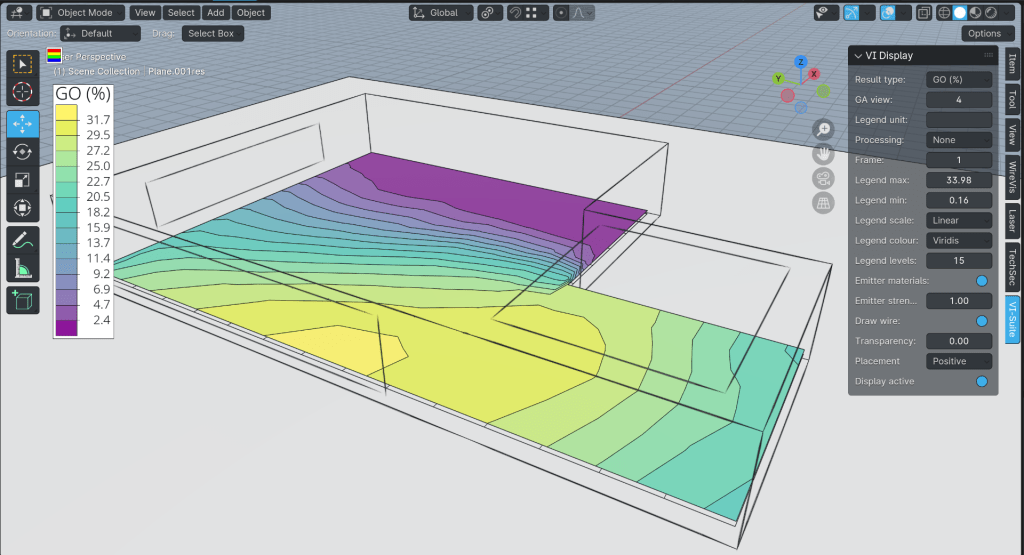
In other news, there are now 2 new experimental display modes for mesh visualisation of results i.e. SVF, Shadow maps and LiVi results. These two modes are Interpolate and Direction and both are exposed as options in the VI-Suite View panel before the visualisation button is clicked.

Interpolate does what it says on the packet and uses matplotlib to interpolate the results on the mesh. There are however limitations to this approach as matplotlib only does 2D interpolation so the sensor mesh should also be 2D. The sensor mesh can be moved and rotated but the transforms should not be cleared in Blender – the results mesh will likely appear in the wrong place if you do.

Another limitation with interpolation is that point numerical visualisation is not available as the results mesh is now a completely new mesh and not based on the sensor mesh. Also, as the interpolation is based on sensor mesh vertex position, then using vertices as the sensor point creates a more accurate interpolation.

Finally, there is a new option in the view panel which is Placement. This is required as Blender cannot convert the matplotlib interpolations into a mesh fully, but has to create overlapping planes. This means a result band forming one plane can be totally obscured by another when it should be visible. The Placement option orders the position of each result band in either result value order or reverse result value order so this may need to be changed in order to see all result planes as they should be. Even then there can be cases where not all result planes are seen, so interpolate should be used with care.

Interpolation

The second display option is for directional results, which at the moment means annual glare calculations (available in the CBDM menu of the LiVi Context node). Any other king of metric will fail, and the code does not currently check there are annual glare results to visualise and will therefore likely cause an error if not. The Direction visualisation will create an arrow for each face/vertex of the sensor mesh. This arrow is coloured according to the legend, and will point in the direction of the chosen view. Point numerical visualisation works as normal. There is one additional option in the View panel which is Arrow size, and this simply changes the size of the display arrow.

Directional


EnVi also got some love and can now export the Exhaust fan surface flow component to EnergyPlus, and is available in the Surface Flow node.

If these changes break things, and they might well do so, I have created a branch on the download page for Blender 4.1 that does not include these changes.

Enjoy!

Ryan

Blender 4.0

Hello all.

As we can all now tuck into the new features of Blender 4.0, this is just a note to say that due to Blender API changes the VI-Suite github master branch, which has been updated for 4.0, will probably no longer work on 3.6. If you want to use the VI-Suite with Blender 3.6 then use the link to the beta 2 branch on this blog’s download page. This beta 2 branch is however unlikely to see any further changes.

In other news, there is also a draft manual for v0.7 on the documentation page, which is also included in the github master and beta 2 branch download.

Cheers

Ryan


VI Chart updates

Just a quick note to say that I have just committed to master some changes that will break the VI-Chart node in existing files, and you will need to recreate any chart nodes in your node tree. It may also be necessary to recreate some simulation results in order to be able to chart them. If charting climate data you just need to re-select the EPW file in the VI Location node.  LiVi CBDM and EnVi analyses will need to be re-simulated. Other simulations should be OK.

Sorry for any inconvenience but the implementation is now much simpler and easier to maintain.

Ryan


VI-Suite v0.7 – De-noising Radiance Images

As v0.7 slowly stabilises I’m kicking off the tutorial series with a look at de-noising Radiance images generated with LiVi.

Blender has a nice image de-noising capability that can be used quite effectively with Radiance images. De-noising does not replace higher accuracy analyses – ‘Low’ accuracy settings will still generally produce overall lower luminance and illuminance values, especially in interior scenes – but this is a nice trick to get cleaner images with reduced simulation time.

De-noise comparison

Comparison between the original rpict image and it’s de-noised version

Bug reports and questions can be posted on the Google Group.

Video tutorial is below.

VI-Suite v0.7 – Testing required

Before anyone gets too excited I have not released v0.7 yet. Still working on some features. There is however a new installation procedure that requires some testing.

VI-Suite v0.7 no longer includes all the required Python libraries such as matplotlib and kivy, but uses pip to install them when the addon is activated. This has the advantage that the VI-Suite download is much smaller, but more importantly I don’t have to update all the libraries when Blender changes its Python version.

To test this new install mechanism with Blender 3.3 get the zip file from https://github.com/rgsouthall/vi-suite07/archive/refs/heads/master.zip and install from the preferences addon menu as normal. Assuming you have a live internet connection there will then be a pause as the libraries are downloaded. On a slow internet connection this can take some time although this only happens the first time the addon is activated. If you start Blender from a terminal, or show the terminal window on Windows, you can monitor the installation process.

Assuming install completes, then try a simple chart display to test matplotlib and a simulation that takes enough time to bring up the progress window to test Kivy. Any successes or failures, with platform information and any error messages, can be reported as a comment below.

Cheers

Ryan

VI-Suite 0.6.1 – Call for testing

Dear all.

The Vi-Suite (v0.6.1) has been updated to work with the current Blender 2.93LTS release. I have not however had a lot of time for bug hunting so some testing, especially on Windows and OS X platforms, is still required.

There are no major changes in this release except for the update to the newer Blender version. I have however made some changes to the VI Location, LiVi Context, EnVi Context, EnVi Sub-surface flow and EnVi Opaque layer nodes that will mean these nodes will have to be recreated if updating a v0.6 analysis to a v0.6.1 one.

General questions can go on the Google Group https://groups.google.com/g/vi-suite and bug reports can be filed at https://github.com/rgsouthall/vi-suite061/issues. Bug reports should contain information regarding operating system, method of install, and any relevant terminal output and/or contents of the vi-suite-log file. Images of node setups can also be useful.

v0.6.1 sits now in its own github repository which can be found at https://github.com/rgsouthall/vi-suite061 and the current master version can be downloaded from https://github.com/rgsouthall/vi-suite061/archive/refs/heads/master.zip.

Enjoy.

Ryan

VI-Suite v0.6 – Basic OpenFOAM analysis

Hello again.

I’ve just uploaded a video on how to use the FloVi component of the VI-Suite to conduct an air-flow simulation with OpenFOAM. The FloVi component only currently works on Linux, and I have only tested it on Arch Linux, but it should work on other Linux distributions.

A FloVi analysis requires as a minimum a manifold mesh object to act as a CFD domain. Additional manifold mesh objects can be added within the domain but geometries cannot overlap as this is not supported by Netgen.

There was a bug in the symmetry boundary specification which I fixed a few days ago so make sure you have a recent version of the VI-Suite v0.6 from github.

The example I show in the video is of a domain with ground terrain making up one of the boundary surfaces. If a building is to be modelled that touches the ground plane then one way is to extrude the shape up from the ground boundary. This way the skin of the building becomes a continuation of the domain boundary.

Extrusion

Extrusion from the ground plane

Another way is to add the building geometry as CFD geometry, but as said earlier this cannot overlap with the domain boundary. One way to get round this is to remove the ground plane that the building sits on, and then fill the edges between the bottom of the walls and the bottom edges of the domain.

A third way is to do a boolean difference between the CFD domain and the building geometry. The example below shows a boolean difference operation between the domain and an overlapping torus, which leaves the torus shape as a perturbation to the ground plane.

Boolean difference

Generating boundary geometry with a boolean difference

FloVi is experimental and generally works for me, but is not meant to intelligently apply boundary conditions for you. That is a manual process, and you should know what boundary conditions are appropriate for the simulation context you have. If the interface does not write out the correct boundary information based on your input then file a bug report at the github page and if there are additional boundary conditions you want added to the interface then post a request on the Google Group.

The default OpenFOAM solver I use in the video is simpleFOAM, and this is the one I’ve got working fairly reliably.

Finally, although the VI-Suite itself cannot visualise OpenFOAM results there is another another Blender node-based addon called BVTKNodes that can open OpenFOAM meshes and results and I have had some joy visualising results with it, so check it out if you want a complete Blender workflow.

That’s it I think. As ever, video below.