Hello.
I had to make a slight change to make the VI-Suite compatible with Blender 4.1 but I haven’t noticed any other problems.
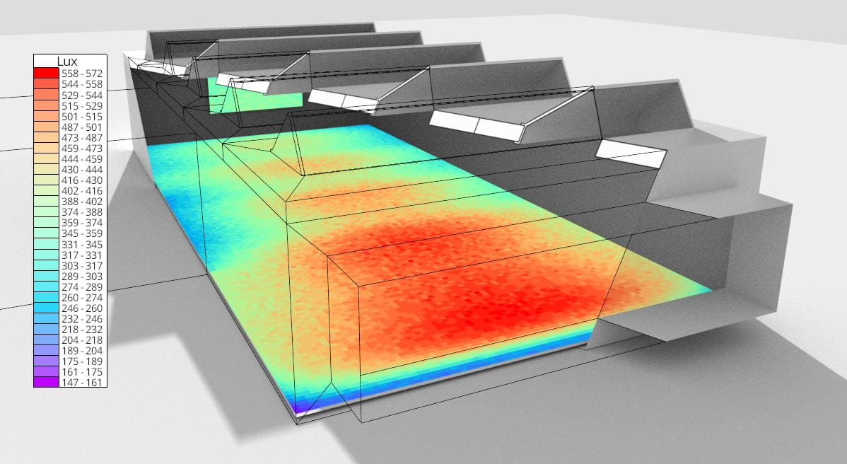
In other news, there are now 2 new experimental display modes for mesh visualisation of results i.e. SVF, Shadow maps and LiVi results. These two modes are Interpolate and Direction and both are exposed as options in the VI-Suite View panel before the visualisation button is clicked.
Interpolate does what it says on the packet and uses matplotlib to interpolate the results on the mesh. There are however limitations to this approach as matplotlib only does 2D interpolation so the sensor mesh should also be 2D. The sensor mesh can be moved and rotated but the transforms should not be cleared in Blender – the results mesh will likely appear in the wrong place if you do.
Another limitation with interpolation is that point numerical visualisation is not available as the results mesh is now a completely new mesh and not based on the sensor mesh. Also, as the interpolation is based on sensor mesh vertex position, then using vertices as the sensor point creates a more accurate interpolation.
Finally, there is a new option in the view panel which is Placement. This is required as Blender cannot convert the matplotlib interpolations into a mesh fully, but has to create overlapping planes. This means a result band forming one plane can be totally obscured by another when it should be visible. The Placement option orders the position of each result band in either result value order or reverse result value order so this may need to be changed in order to see all result planes as they should be. Even then there can be cases where not all result planes are seen, so interpolate should be used with care.
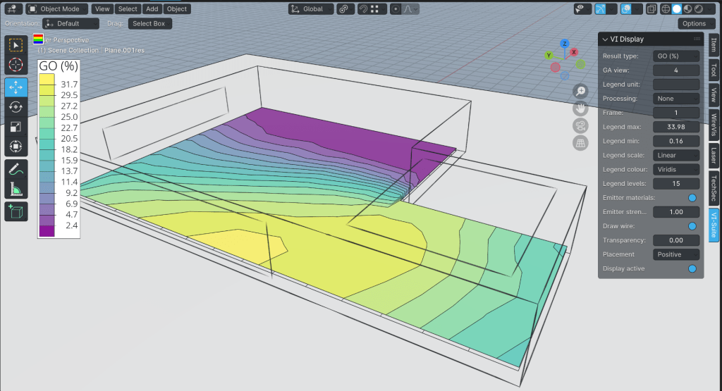
The second display option is for directional results, which at the moment means annual glare calculations (available in the CBDM menu of the LiVi Context node). Any other king of metric will fail, and the code does not currently check there are annual glare results to visualise and will therefore likely cause an error if not. The Direction visualisation will create an arrow for each face/vertex of the sensor mesh. This arrow is coloured according to the legend, and will point in the direction of the chosen view. Point numerical visualisation works as normal. There is one additional option in the View panel which is Arrow size, and this simply changes the size of the display arrow.

EnVi also got some love and can now export the Exhaust fan surface flow component to EnergyPlus, and is available in the Surface Flow node.
If these changes break things, and they might well do so, I have created a branch on the download page for Blender 4.1 that does not include these changes.
Enjoy!
Ryan