
x = a:dx:b
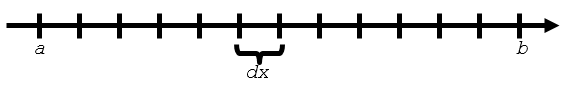 When element spacing
 dx is known.
x = linspace(a,b,n)
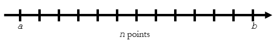 When number of elements
 n is known.
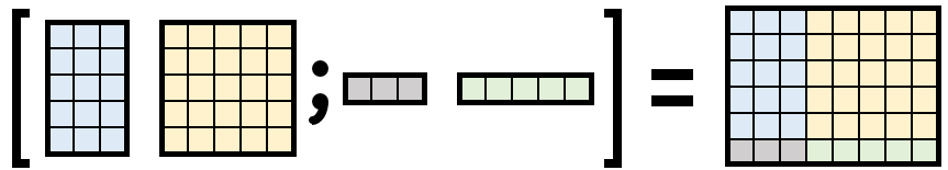
x(:).Concatenating Arrays
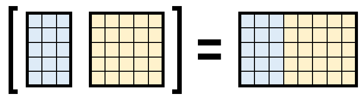
Horizontal Concatenation
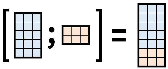
Vertical Concatenation
Combined Concatenation
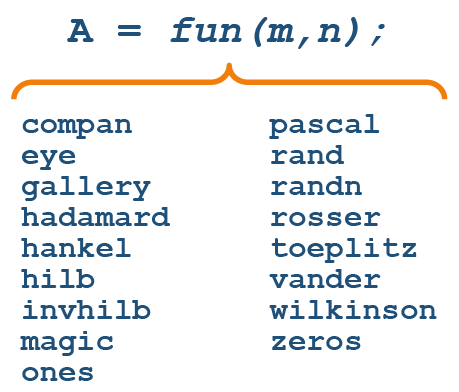
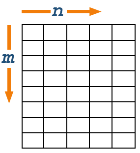
Array Creation Functions
 |
 |
|
For convenience, you can also leave one of the dimensions blank when calling
reshape and that dimension will be calculated automatically. |
|
y = reshape(x,5,[]); |
If you want to remove elements from a vector, you can do so by assigning
v = [1 2 3 4 5];
v([2 4]) = []
    [1 3 5]
Summary: Accessing Data in Arrays
Indexing


|
Extract one element from a vector
|
|
v(2) 1.5
|
|||
|
Extract the last element from a vector
|
|
v(end) 1.3
|
|||
|
Extract multiple elements from a vector
|
|
v([1 end-2:end]) 2.3 1.3 0.9 1.3 |
When you are extracting elements of a matrix you need to provide two indices, the row and column numbers.
|
Extract one element from a matrix
|
|
M(2,3) 1.7
|
|||
|
Extract an entire column. Here, it is the last one.
|
|
M(:,end) 0.9 1.4 0.7 2.5 0.6 |
|||
|
Extract multiple elements from a matrix.
|
|
M([1 end],2) 1.1 2.8 |
Changing Elements in Arrays
|
Change one element from a vector
|
|
v(2) = 0 2.3 0 1.3 0.9 1.3 |
|||
|
Change multiple element of a vector to the same value
|
|
v(1:3) = 0 0 0 0 0.9 1.3 |
|||
|
Change multiple element of a vector to different values
|
|
v(1:3) = [3 5 7] 3 5 7 0.9 1.3 |
|||
|
Assign a non-existent value
|
|
v(9) = 42 3 5 7 0.9 1.3 0 0 0 42 |
|||
|
Remove elements from a vector
|
|
v(1:3) = [] 0.9 1.3 0 0 0 42 |
Changing elements in matrices works the same way as with vectors, but you must specify both rows and columns.
Introduction to Matrix Multiplication
You have done element-wise arithmetic, including multiplication (.*). There is another way to multiply matrices, called matrix multiplication (*). It is the same matrix multiplication taught in linear algebra. You can think of it as a way to add elements in a row where you weight, or scale, the elements differently.
Weighted Sums
A weighted sum is where you scale numbers then add them together.
One example of this is how some teachers calculate final grades. If tests are worth 50% of the final grade, homework is 40%, and quizzes are 10%, then a student’s grades are calculated by multiplying these proportions by the test, homework, and quiz grades and adding them together.

Matrix-Vector Multiplication
Matrix multiplication of a matrix times a vector is the weighted sum of each row of the matrix.
So, imagine a teacher records the test, homework, and quiz scores of different students in the rows of a matrix. Multiplying the matrix of grades times the vector of weights, gives you the grades for each student.

Matrix-Matrix Multiplication
When multiplying two matrices, the elements of the resutling matrix are the weighted sums of the rows and columns of the first and second matrix, respectively. Note that the matrix order is important since matrix multiplication is not commutative. That is,
.


Matrix Dimensions
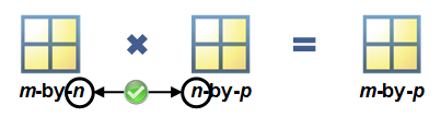
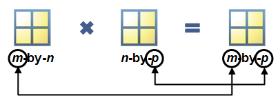
Matrix multiplication requires that the dimensions agree. You need the same number of columns in the first matrix as there are rows in the second, or there won’t be enough elements to multiply together.

Matrix multiplication requires that the inner dimensions of the two matrices agree. The resulting matrix has the outer dimensions of the two matrices.

x is a 2-by-3 matrix. |
|
x = [1 0 7 ; 3 2 5] x = 1 0 7 3 2 5 |
|||
y is a 3-by-4 matrix. |
|
y = [0 4 2 1 ; 2 1 0 2 ; 1 3 1 0] y = 0 4 2 1 2 1 0 2 1 3 1 0 |
|||
|
The result
z is a 2-by-4 matrix. |
|
z = x*y z = 7 25 9 1 9 29 11 7 |
Summary: Mathematical and Statistical Operations with Arrays
Performing Operations on Arrays
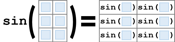
There are many operators that behave in element-wise manner, i.e., the operation is performed on each element of the array individually.
Mathematical Functions
| Other Similar Functions | |
|---|---|
sin |
Sine |
cos |
Cosine |
log |
Logarithm |
round |
Rounding Operation |
sqrt |
Square Root |
mod |
Modulus |
| Many more | |
Matrix Operations (Including Scalar Expansion)
| Operators | |
|---|---|
+ |
Addition |
- |
Subtraction |
* |
Multiplication |
/ |
Division |
^ |
Exponentiation (Matrix exponentiation) |
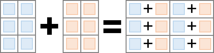
Element-wise Operations
| Operators | |
|---|---|
+ |
Addition |
- |
Subtraction |
.* |
Element-wise Multiplication |
./ |
Element-wise Division |
.^ |
Element-wise Exponentiation |
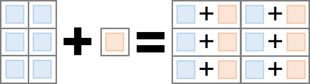
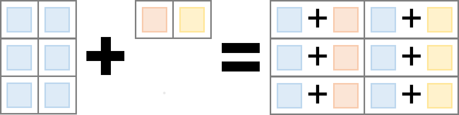
Implicit Expansion
| Operators | |
|---|---|
+ |
Addition |
- |
Subtraction |
.* |
Element-wise Multiplication |
./ |
Element-wise Division |
.^ |
Element-wise Exponentiation |
Calculating Statistics of Vectors
Common Statistical Functions
| Function | Description |
|---|---|
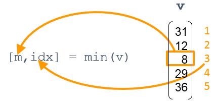
min |
Returns the minimum element |
max |
Returns the maximum element |
mean |
Returns the average of the elements |
median |
Returns the median value of the elements |
Using min and max
Ignoring NaNs
When using statistical functions, you can ignore NaN values
avg = mean(v,"omitnan")
Statistical Operations on Matrices
| Function | Behavior |
|---|---|
max |
Largest elements |
min |
Smallest elements |
mean |
Average or mean value |
median |
Median value |
mode |
Most frequent values |
std |
Standard deviation |
var |
Variance |
sum |
Sum of elements |
prod |
Product of elements |
A = [8 2 4 ; 3 2 6 ; 7 5 3 ; 7 10 8] A = 8 2 4 3 2 6 7 5 3 7 10 8 |
||
Amax = max(A) Amax = 8 10 8 |
||
Astd = std(A) Astd = 2.2174 3.7749 2.2174 |
||
Asum = sum(A) Asum = 25 19 21 |
>>
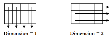
= mean(A,dim)
M |
Vector of average values along dimension dim. |
A |
Matrix |
dim |
Dimension across which the mean is taken.1: the mean of each column2: the mean of each row |
Matrix Multiplication
Matrix multiplication requires that the inner dimensions agree. The resultant matrix has the outer dimensions.

Solving Systems of Linear Equations
| Expression | Interpretation |
|---|---|
x = B/A |
Solves x*A=B (for x) |
x = A\B |
Solves A*x=B (for x) |
Summary: Tables of Data
Storing Data in a Table
|
The
readtable function creates a table in MATLAB from a data file. |
|
EPL = readtable("EPLresults.xlsx","TextType","string"); |
|||
|
The
table function can create a table from workspace variables. |
|
teamWinsTable = table(team,wins) teamWins = Team Wins ___________________ ____ "Arsenal" 20 "Chelsea" 12 "Leicester City" 23 "Manchester United" 19 |
|||
|
The
array2table function can convert a numeric array to a table. The VariableNames property can be specified as a string array of names to include as variable names in the table. |
|
stats = array2table(wdl, ...
    "VariableNames",["Wins" "Draws" "Losses"])
stats = Wins Draws Losses ____ _____ ______ 20 11 7 12 14 12 23 12 3 19 9 10 |
Sorting Table Data
|
The
sortrows function sorts the data in ascending order, by default. |
|
EPL = sortrows(EPL,"HomeWins"); |
|||
|
Use the optional
"descend" parameter to sort the list in descending order. |
|
EPL = sortrows(EPL,"HomeWins","descend"); |
|||
|
You can also sort on multiple variables, in order, by specifying a string array of variable names.
|
|
EPL = sortrows(EPL,["HomeWins" "AwayWins"],"descend"); |
|||
|
You can also show
summary statistics for variables in a table. |
|
summary(EPL) |
Extracting Portions of a Table
|
Display the original table.
|
|
EPL
EPL = Team HW HD HL AW AD AL ___________________ __ __ __ __ __ __ "Leicester City" 12 6 1 11 6 2 "Arsenal" 12 4 3 8 7 4 "Manchester City" 12 2 5 7 7 5 "Manchester United" 12 5 2 7 4 8 "Chelsea" 5 9 5 7 5 7 "Bournemouth" 5 5 9 6 4 9 "Aston Villa" 2 5 12 1 3 15 |
|||
|
Inside parenthesis, specify the row numbers of the observations and column numbers of the table variables you would like to select.
|
|
EPL(2:4,[1 2 5]) ans = Team HW AW ___________________ __ __ "Arsenal" 12 8 "Manchester City" 12 7 "Manchester United" 12 7 |
|||
|
You may also use the name of the variable for indexing. If you want to reference more than one variable, use a string array containing the variable names. |
|
EPL(2:4,["Team" "HW" "AW"]) ans = Team HW AW ___________________ __ __ "Arsenal" 12 8 "Manchester City" 12 7 "Manchester United" 12 7 |
Extracting Data from a Table
|
Display the original table.
|
|
EPL
EPL = Team HW HD HL AW AD AL ___________________ __ __ __ __ __ __ "Leicester City" 12 6 1 11 6 2 "Arsenal" 12 4 3 8 7 4 "Manchester City" 12 2 5 7 7 5 "Manchester United" 12 5 2 7 4 8 |
|||
|
You can use dot notation to extract data for use in calculations or plotting.
|
|
tw = EPL.HW + EPL.AW tw = 23 20 19 19 |
|||
|
You can also use dot notation to create new variables in a table.
|
|
EPL.TW = EPL.HW + EPL.AW EPL = Team HW HD HL AW AD AL TW ___________________ __ __ __ __ __ __ __ "Leicester City" 12 6 1 11 6 2 23 "Arsenal" 12 4 3 8 7 4 20 "Manchester City" 12 2 5 7 7 5 19 "Manchester United" 12 5 2 7 4 8 19 |
|||
|
If you want to extract multiple variables, you can do this using curly braces.
|
|
draws = EPL{:,["HD" "AD"]} draws = 6 6 4 7 2 7 5 4 |
|||
|
Specify row indices to extract specific rows.
|
|
draws13 = EPL{[1 3],["HD" "AD"]} draws = 6 6 2 7 |
Exporting Tables
You can use the writetable function to create a file from a table.
writetable(tableName,"myFile.txt","Delimiter","\t")
The file format is based on the file extension, such as .txt, .csv, or .xlsx, but you can also specify a delimiter.
Summary: Organizing Tabular Data
Combining Tables
If the tables are already aligned so that the rows correspond to the same observation, you can concatenate them with square brackets.
[teamInfo games]

If the tables are not already aligned so that the rows correspond to the same observation, you can still combine the data by merging them with a join.

|
The
join function can combine tables with a common variable. |
|
top3 = join(uswntTop3,posTop3) top3 = Player Goals Position ___________________ ______ ___________________ "Alex Morgan" 6 "forward" "Megan Rapinoe" 6 "forward" "Rose Lavelle" 3 "midfielder" |
Table Properties
|
Display the table properties.
|
|
EPL.Properties
ans = Table Properties with properties: Description: '' UserData: [] DimensionNames: {'Row' 'Variable'} VariableNames: {1×11 cell} VariableDescriptions: {1×11 cell} VariableUnits: {} VariableContinuity: [] RowNames: {} CustomProperties: No custom properties are set. |
|||
|
You can access an individual property of
Properties using dot notation. |
|
EPL.Properties.VariableNames
ans = 1×11 cell array Columns 1 through 4 {'Team'} {'HomeWins'} {'HomeDraws'} {'HomeLosses'} Columns 5 through 8 {'HomeGF'} {'HomeGA'} {'AwayWins'} {'AwayDraws'} Columns 9 through 11 {'AwayLosses'} {'AwayGF'} {'AwayGA'} |
Indexing into Cell Arrays
|
The variable
varNames is a cell array that contains character arrays of different lengths in each cell. |
|
varNames = teamInfo.Properties.VariableNames
|
||||||||||
|
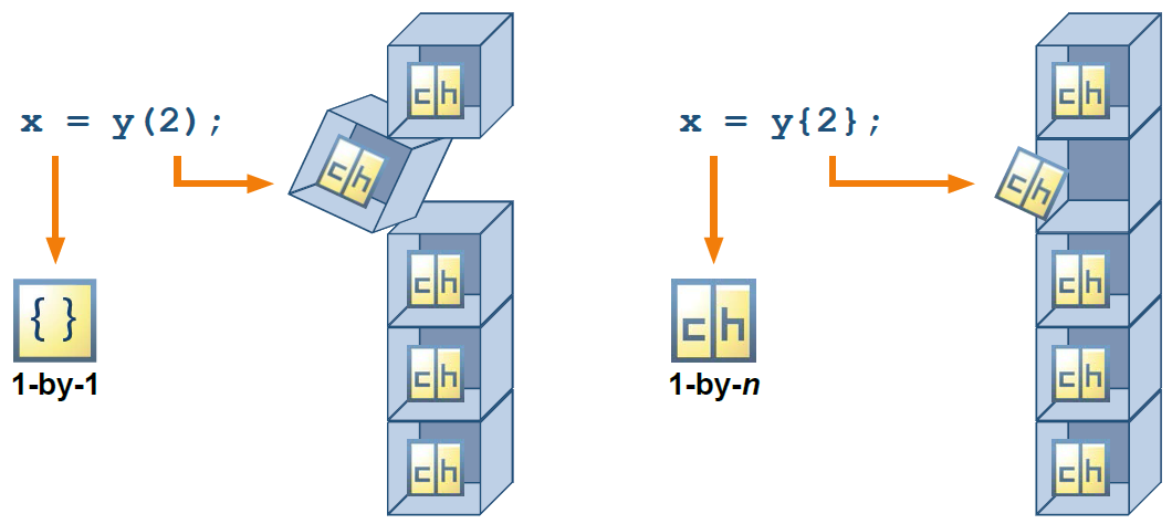
Using parentheses to index produces a cell array, not the character array inside the cell.
|
|
varName(2)
|
||||||||||
|
In order to extract the contents inside the cell, you should index using curly braces,
{}. |
|
varName{2}
|
||||||||||
|
Using curly braces allows you to rename the variable.
|
|
varName{2} = 'Payroll'
|
Summary: Specialized Data Types
Working with Dates and Times
|
Dates are often automatically detected and brought in as
datetime arrays. |
|
teamInfo
ans = Manager ManagerHireDate _________________ _______________ "Rafael Benítez" 3/11/2016 "Claudio Ranieri" 7/13/2015 "Ronald Koeman" 6/16/2014 "David Unsworth" 5/12/2016 "Slaven Bilić" 6/9/2015 |
|||
|
Many functions operate on datetime arrays directly, such as
sortrows. |
|
sortrows(teamInfo,"ManagerHireDate") ans = Manager ManagerHireDate _________________ _______________ "Ronald Koeman" 6/16/2014 "Slaven Bilić" 6/9/2015 "Claudio Ranieri" 7/13/2015 "Rafael Benítez" 3/11/2016 "David Unsworth" 5/12/2016 |
|||
|
You can create a
datetime array using numeric inputs. The first input is year, then month, then day. |
|
t = datetime(1977,12,13) t = 13-Dec-1977 |
|||
|
To create a vector, you can specify an array as input to the
datetime function. |
|
ts = datetime([1903;1969],[12;7],[17;20]) ts = 17-Dec-1903 20-Jul-1969 |
Operating on Dates and Times
|
Create
datetime variables to work with. |
|
seasonStart = datetime(2015,8,8) seasonStart = 08-Aug-2015 seasonEnd = datetime(2016,5,17) seasonEnd = 17-May-2016 |
|||
|
Use subtraction to produce a
duration variable. |
|
seasonLength = seasonEnd - seasonStart seasonLength = 6792:00:00 |
|||
|
|
seasonLength = days(seasonLength) seasonLength = 283 |
||||
|
They can also create durations from a numeric value.
|
|
seconds(5) ans = 5 seconds |
|||
|
Use the
between function to produce a context-dependent calendarDuration variable. |
|
seasonLength = between(seasonStart,seasonEnd) seasonLength = 9mo 9d |
|||
|
|
calmonths(2) ans = 2mo |
You can learn more about datetime and duration functions in the documentation.
Create Date and Time Arrays
Representing Discrete Categories
x is a string array. |
|
x = ["C" "B" "C" "A" "B" "A" "C"]; x = "C" "B" "C" "A" "B" "A" "C" |
|||
|
|
y = categorical(x); y = C B C A B A C |
||||
|
You can use
== to create a logical array, and count elements using nnz. |
|
nnz(x == "C") ans = 3 |
|||
|
You can view category statistics using the
summary function. |
|
summary(y) A B C 2 2 3 |
|||
|
You can view combine categories using the
mergecats function. |
|
y = mergecats(y,["B" "C"],"D") y = D D D A D A D |
Summary: Preprocessing Data
Normalizing Data
|
Normalize the columns of a matrix using z-scores.
|
|
xNorm = normalize(x) |
|||
|
Center the mean of the columns in a matrix on zero.
|
|
xNorm = normalize(x,"center","mean") |
|||
|
Scale the columns of a matrix by the first element of each column.
|
|
xNorm = normalize(x,"scale","first") |
|||
|
Stretch or compress the data in each column of a matrix into a specified interval.
|
|
xNorm = normalize(x,"range",[a b]) |
Working with Missing Data
Any calculation involving NaN results in NaN. There are three ways to work around this, each with advantages and disadvantages:
| Ignore missing data when performing calculations. | Maintains the integrity of the data but can be difficult to implement for involved calculations. |
| Remove missing data. | Simple but, to keep observations aligned, must remove entire rows of the matrix where any data is missing, resulting in a loss of valid data. |
| Replace missing data. | Keeps the data aligned and makes further computation straightforward, but modifies the data to include values that were not actually measured or observed. |
The Clean Missing Data task can be used to remove or interpolate missing data. You can add one to a script by selecting it from the Live Editor tab in the toolstrip.

|
Data contains missing values, in the form of both
-999 and NaN. |
|
x = [2 NaN 5 3 -999 4 NaN]; |
|||
|
The
ismissing function identifies only the NaN elements by default. |
|
ismissing(x) ans = 1×7 logical array 0 1 0 0 0 0 1 |
|||
|
Specifying the set of missing values ensures that
ismissing identifies all the missing elements. |
|
ismissing(x,[-999,NaN]) ans = 1×7 logical array 0 1 0 0 1 0 1 |
|||
|
Use the
standardizeMissing function to convert all missing values to NaN. |
|
xNaN = standardizeMissing(x,-999) xNaN = 2 NaN 5 3 NaN 4 NaN |
|||
|
Use the
rmmissing function to remove missing values. |
|
cleanX = rmmissing(xNaN) cleanX = 2 5 3 4 |
Ignores NaNs by default(default flag is "omitnan") |
Includes NaNs by default(default flag is "includenan") |
|---|---|
maxmin |
covmeanmedianstdvar |
| Data Type | Meaning of “Missing” |
|---|---|
doublesingle |
NaN |
string array |
Empty string (<missing>) |
datetime |
NaT |
durationcalendarDuration |
NaN |
categorical |
<undefined> |
Interpolating Missing Data
|
Interpolation assuming equal spacing of observations.
|
|
z = fillmissing(y,"method") |
|||
|
Interpolation with given observation locations.
|
|
z = fillmissing(y,"method","SamplePoints",x) |
| Method | Meaning |
|---|---|
"next" |
The missing value is the same as the next nonmissing value in the data. |
"previous" |
The missing value is the same as the previous nonmissing value in the data. |
"nearest" |
The missing value is the same as the nearest (next or previous) nonmissing value in the data. |
"linear" |
The missing value is the linear interpolation (average) of the previous and next nonmissing values. |
"spline" |
Cubic spline interpolation matches the derivatives of the individual interpolants at the data points. This results in an interpolant that is smooth across the whole data set. However, this can also introduce spurious oscillations in the interpolant between data points. |
"pchip" |
The cubic Hermite interpolating polynomial method forces the interpolant to maintain the same monotonicity as the data. This prevents oscillation between data points. |
Summary: Common Data Analysis Techniques
Moving Window Operations
The Smooth Data task can be used to smooth variation or noise in data. You can add one to a script by selecting it from the Live Editor tab in the toolstrip.

The Smooth Data task uses the smoothdata function.
|
Mean calculated with a centered moving k-point window.
|
|
z = smoothdata(y,"movmean",k) |
|||
|
Mean calculated with a moving window with kb points backward and kf points forward from the current point.
|
|
z = smoothdata(y,"movmean",[kb kf]) |
|||
|
Median calculated with a centered moving k-point window.
|
|
z = smoothdata(y,"movmedian",k) |
|||
|
Median calculated with a centered moving k-point window using sample points defined in
x. |
|
z = smoothdata(y,"movmedian",k,"SamplePoints",x) |
Linear Correlation
You can investigate relationships between variables visually and computationally:
- Plot multiple series together. Use
yyaxisto add another vertical axis to allow for different scales. - Plot variables against each other. Use
plotmatrixto create an array of scatter plots. - Calculate linear correlation coefficients. Use
corrcoefto calculate pairwise correlations.
|
Plot multiple series together.
|
|
yyaxis left plot(...) yyaxis right plot(...) 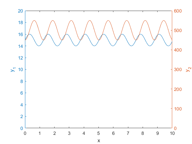 |
|||
|
Plot variables against each other.
|
|
plotmatrix(data) 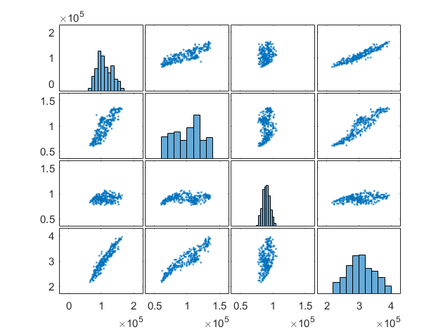 |
|||
|
Calculate linear correlation coefficients.
|
|
corrcoef(data) ans = 1.0000 0.8243 0.1300 0.9519 0.8243 1.0000 0.1590 0.9268 0.1300 0.1590 1.0000 0.2938 0.9519 0.9268 0.2938 1.0000 |
Polynomial Fitting
Simple fitting
|
Fit polynomial to data.
|
|
c = polyfit(x,y,n); |
|||
|
Evaluate fitted polynomial.
|
|
yfit = polyval(c,xfit); |
Fitting with centering and scaling
|
Fit polynomial to data.
|
|
[c,~,scl] = polyfit(x,y,n); |
|||
|
Evaluate fitted polynomial.
|
|
yfit = polyval(c,xfit,[],scl); |
Summary: Programming Constructs
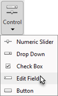
User Interaction
|
You can add a live control to get input from the user.
|
|
 |
|||
|
You can use
disp to show output on the command window. |
|
disp("Message") Message
|
|||
|
|
warning("Missing data") Warning: Missing data error("Missing data") Missing data |
||||
|
|
msgbox("Analysis complete") 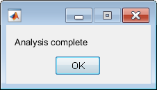 |
Decision Branching
|
The
condition_1 is evaluated as true or false. |
|
if condition_1 |
|||
|
If
condition_1 is true, then the code_1 code block is executed. |
|
code_1
|
|||
|
Otherwise, the next case is tested. There can be any number of cases.
|
|
elseif condition_2 code_2 elseif condition_3 code_3 |
|||
|
If none of the cases are a match, then the code,
code_e, in else is executed. |
|
else code_e |
|||
|
Always end the expression with the keyword
end |
|
end
|
|
Evaluate
expression to return a value. |
|
switch expression |
|||
|
If
expression equals value_1, then code_1 is executed. Otherwise, the next case is tested. There can be any number of cases. |
|
case value 1 code_1 case value 2 code_2 |
|||
|
If none of the cases are a match, then the code,
code_3, in otherwise is executed. The otherwise block is optional. |
|
otherwise code_3 |
|||
|
Always end the expression with the keyword
end |
|
end
|
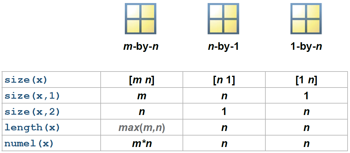
Determining Size
|
Use
size to find the dimensions of a matrix. |
|
s = size(prices) s = 19 10 [m,n] = size(prices) m = 19 n = 10 m = size(prices,1) m = 19 n = size(prices,2) n = 10 |
|||
|
|
m = length(Year) m = 19 |
||||
|
Use
numel to find the total number of elements in an array of any dimension. |
|
N = numel(prices) N = 190 |
For Loops
|
The index is defined as a vector. Note the use of the colon syntax to define the values that the index will take.
|
|
for index = first:increment:last code end |
While Loops
|
The condition is a variable or expression that evaluates to
true or false. While condition is true, code executes. Once condition becomes false, the loop ceases execution. |
|
while condition code end |
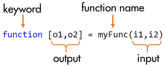
Summary: Increasing Automation with Functions
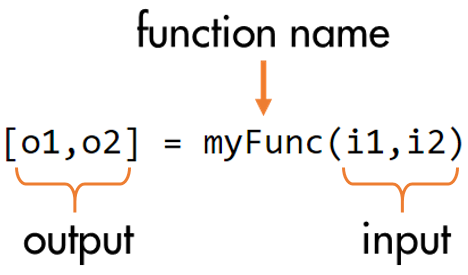
Creating and Calling Functions
| Define a function | Call a function |
|---|---|
 |
 |
Function Files
| Function Type | Function Visibility |
|---|---|
| Local functions: Functions that are defined within a script. |
Visible only within the file where they are defined. |
| Functions: Functions that are defined in separate files. |
Visible to other script and function files. |
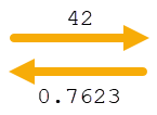
Workspaces
A function maintains its own workspace to store variables created in the function body.
a = 42; b = foo(a);
|
 |
foo.mlx
|
||||||||||||||||
|
|
|||||||||||||||||
 a
aMATLAB Path and Calling Precedence
In MATLAB, there are rules for interpreting any named item. These rules are referred to as the function precedence order. Most of the common reference conflicts can be resolved using the following order:
- Variables
- Functions defined in the current script
- Files in the current folder
- Files on MATLAB search path
A more comprehensive list can be found here.
The search path, or path is a subset of all the folders in the file system. MATLAB can access all files in the folders on the search path.
To add folders to the search path:
- On the Home tab, in the Environment section, click Set Path.
- Add a single folder or a set of folders using the buttons highlighted below.
